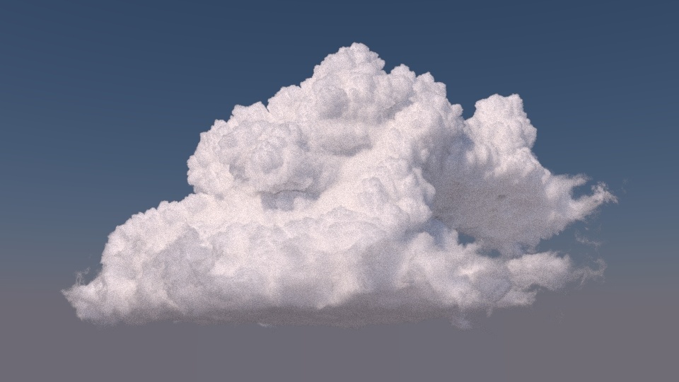
 The Moana Cloud asset rendered using the Aggregate Volumes workflow. OpenVDB Asset courtesy of Walt Disney Animation. CC BY-SA 3.0 License.
When rendering clouds with the Aggregate Volumes workflow, there are a number of key settings that you can adjust to control the look of a cloud. All images on this page were rendered using a scene set up in RfM. Instructions for setting up the scene can be found in the Scene Setup sectionThis document outlines aggregate volume controls in the context of rendering clouds.
Volume Settings
Max Path Length
The max path length is an extremely important control when rendering clouds. A relatively high maximum path length is required to achieve a cloudlike appearance. The images below are rendered with max path lengths of 0, 16, and 64, respectively.
| Carousel Image Slider | ||||||||||||||||
|---|---|---|---|---|---|---|---|---|---|---|---|---|---|---|---|---|
| ||||||||||||||||
| Gallery | ||||||||||||||||
|
The change at higher path lengths is more subtle, but in order to get noticeable light bleed in shadowed areas of the cloud, a very high maximum path length is needed.
| Before After Image Slider | ||||||||||||
|---|---|---|---|---|---|---|---|---|---|---|---|---|
|
The cloud scene rendered with path lengths of 64 (left) and 256 (right).
| Tip |
|---|
Increasing the max path length also increases render times, so you should keep it as low as possible. Multi-Scattering Approximation (outlined below) can help mimic high path lengths at much lower cost. |
...
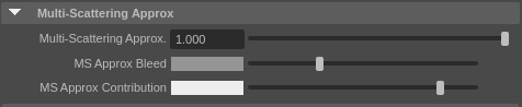
The Multi-Scattering Approximation (MS Approx) settings are a group of settings that mimic the effect of multi-scattering within a volume. When set correctly, MS Approx can produce a similar look to very high path lengths, but without increasing render times. There are three MS Approx controls, Multi-Scattering ApproximationApprox., MS Approx Bleed, and MS Approx Contribution. The effect of each setting is outlined in the sections below. Although Bleed and Contribution are both colors, the sections below refer to them by a single value which is used for red, green, and blue.
...
| Before After Image Slider | ||||||||||||
|---|---|---|---|---|---|---|---|---|---|---|---|---|
|
The cloud scene rendered with Multi-Scattering Approx. set to 0 (left) and 1 (right) with default Bleed and Contribution.
| Warning |
|---|
Setting Multi-Scattering Approx to values other than 0 or 1 may not produce visually correct images |
MS Approx Bleed
The MS Approx Bleed parameter controls how much light bleeds through a volume. Higher Bleed values allow more light to pass through the volume and light areas that would otherwise be shadowed. As such, the effect of MS Approx Bleed is most visible in shadowed areas of a volume, but it also creates a slight overall brightening effect. You can use the bleed parameter to compensate for the overall loss of brightness caused by lower Max Path Lengths.
| Before After Image Slider | ||||||||||||
|---|---|---|---|---|---|---|---|---|---|---|---|---|
|
The cloud scene rendered with Bleed set to 0.1 (left) and 0.9 (right) with default Contribution.
...
MS Approx Contribution
The MS Approx Contribution parameter controls how much the light bleed from the Bleed parameter contributes to the brightness of the volume. Increasing Contribution tends to increase the overall brightness of the cloud, but it brightens fringes slightly less. You can use the Contribution to help bring out detail along the edges of a volume.
| Before After Image Slider | ||||||||||||
|---|---|---|---|---|---|---|---|---|---|---|---|---|
|
The cloud scene rendered with Contribution set to 0.25 (left) and 0.75 (right) with default Bleed.
MS Approx Suggestions
- It can be tricky to find good values of Bleed and Contribution since they are very dependent on each other. One process you can try is to start by setting Multi-Scattering Approx to 1, then alternate increasing Contribution and decreasing Bleed in small steps until you get the correct balance of brightness in the shadowed areas.
- Contribution tends to produce a stronger brightening effect, so it should be adjusted in smaller increments than Bleed.
- At high values, the Contribution parameter becomes very sensitive, so you should adjust it in small increments (0.05 or less) as it gets close to 1.
...
The density of a cloud has a significant impact on it's appearance. The main control for density is the Density Scale setting on the volume, which scales the density from the input OpenVDB file. Low Density Scale values create an airier, less detailed appearance with more light bleed, while high Density Scale values produce a thicker, more detailed, or even solid appearance.
...
.
...
The images below were rendered with Density Scales of 0.2
...
, 1.0
...
, and 5.0
...
.
| Carousel Image Slider | ||||||||||||||||||
|---|---|---|---|---|---|---|---|---|---|---|---|---|---|---|---|---|---|---|
|
Anisotropy
Adjusting the anisotropy settings in PxrVolume is also critical for getting a realistic cloud render. There are three anisotropy settings to pay attention to, Primary Anisotropy, Secondary Anisotropy, and Lobe Blend Factor. The Primary and Secondary Anisotropy settings control two anisotropic lobes that can be either forward scattering (set to +1) or backward scattering (set to -1). The Lobe Blend controls the relative contribution of the two lobes, where 0 uses only the Primary lobe and 1 uses only the Secondary lobe. Setting the Primary lobe to be forward scattering flattens out detail in some areas of the cloud, but it also adds a darkening effect to parts of the cloud facing the light source.
| Before After Image Slider | ||||||||||||
|---|---|---|---|---|---|---|---|---|---|---|---|---|
|
The cloud scene rendered without anisotropy (left) and with a forward scattering Primary lobe (right) with Primary Anisotropy set to 0.8 and Blend set to 0.
Adding a backward scattering Secondary lobe recovers most of the detail lost in the forward scattering render but still retains some of the detail in the areas facing the light source.
| Before After Image Slider | ||||||||||||
|---|---|---|---|---|---|---|---|---|---|---|---|---|
|
The cloud scene rendered without anisotropy (left) and with a forward scattering Primary lobe and backward scattering Secondary lobe (right) with Primary Anisotropy set to 0.8, Secondary Anisotropy set to -0.2, and Blend set to 0.2.
| Note |
|---|
Enabling anisotropy will introduce additional noise to your render. Higher values of anisotropy will introduce more noise. |
| Anchor | ||||
|---|---|---|---|---|
|
Scene Setup
This section covers how the scene used above was set up in RfM.
...
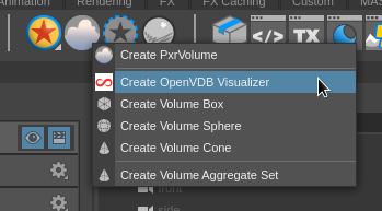
First, create an OpenVDBVisualize object from the RenderMan shelf tab.

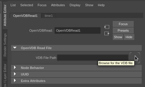
Next, select the VDB file you want to use in the OpenVDBRead settings in the attribute editor (the quarter or eighth resolution versions of the Moana cloud are fine for nowCloud work well for tweaking settings).

Now, you should be able to see a wireframe of the leaf nodes and tiles in the viewport (you may have to zoom out to see the whole cloud). Next, select the OpenVDBVisualize object in the outliner and open the OpenVDBVisualize settings in the attribute editor. Here, we want to you should rotate the volume so that the top of the cloud is in the +Z direction. So, add a 90 degree rotation along the X-axis.


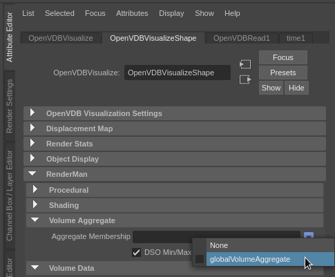
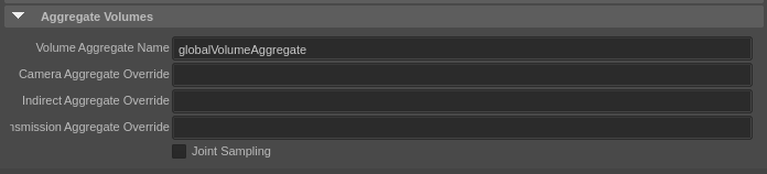
The last thing we want you need to do in the volume settings is add the volume to a volume aggregate. The globalVolumeAggregate is created automatically, so under the OpenVDBVisualizeShape settings, in RenderMan > Volume Aggregate, set the Aggregate Membership to "globalVolumeAggregate".

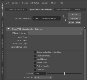
You may also want to disable the visualization of leaf nodes and active tiles, which is under the OpenVDB Visualization Settings.

Volume Shader Settings
In the shader settings, you can also adjust the anisotropy settings under the Anisotropy area. By default, anisotropy is off.


Light Setup
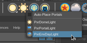
For the light setup, we will use a PxrEnvDayLight. So, the first step in the lighting setup is creating a PxrEnvDayLight from the Renderman tab of the shelf.

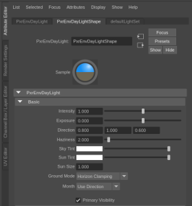
Next, you can adjust the light direction under the PxrEnvDayLightShape tab of the attribut attribute editor either using the Month/Day/Year/Hour (the default method in RfM) or using the Direction control by selecting Month > Use Direction. For To replicate the scene used in this tutorial, we use the direction controls and set the direction to 0.8, 1.0, 0.6. I also found it useful to You should also change the "Ground Mode" from "Legacy" to "Horizon Clamping".

The other defaults provide a good starting point so you can leave them unchanged for now. This is also where you will adjust your MSApprox settings (under Multi-Scatter Approx)Scattering Approximation settings. It can be quite hard to predict how MSApprox MS Approx will affect the render, so you should wait to adjust these settings until after the render is set up completely.
Render Settings
The last thing we you need to tweak before we see our cloud rendered is change to see the rendered clouds are the Render Settings. So, open the Render Settings and select the RenderMan tab. The first thing you should change is under the "Aggregate Volumes" tab. For "Volume Aggregate Name", enter "globalVolumeAggregate" (this is the volume aggregate we added our cloud to before).

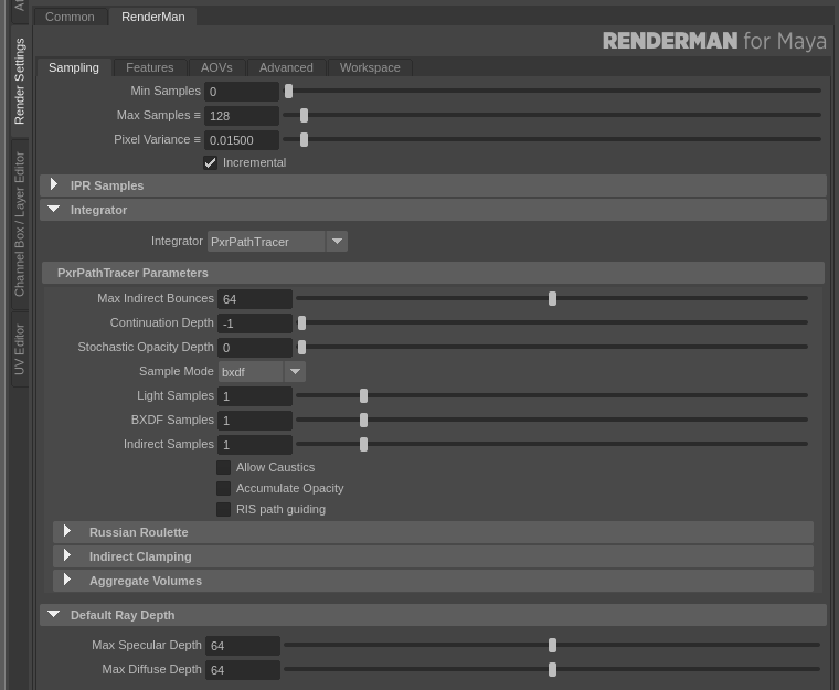
Once you set the volume aggregate name, you should see the cloud if you start a render (either in the viewport or externally in "it"), but it still won't look quite right. To give the cloud the correct appearance, we you need to adjust the number of bounces. First, under "Default Ray Depth", adjust both the "Max Specular Depth" and "Max Diffuse Depth" to much higher values (e.g. no less than 32as described above), and under "PxrPathTracer Parameters", set "Max Indirect Bounces" to that same number.

Multi-
...
Scattering Approx
To begin withadjust the Multi-Scattering Approximation settings, go to the settings on our PxrEnvDayLight and enable MSApprox Multi-Scattering Approximation by setting "Multi-Scatter Scattering Approx" to 1. Now, you can adjust the bleed and contribution as described above. If you find that the cloud is too bright, reducing the value of the MS Approx setting from 1 is an easy way to change the brightness without having to tweak the bleed and contribution too much..

Render
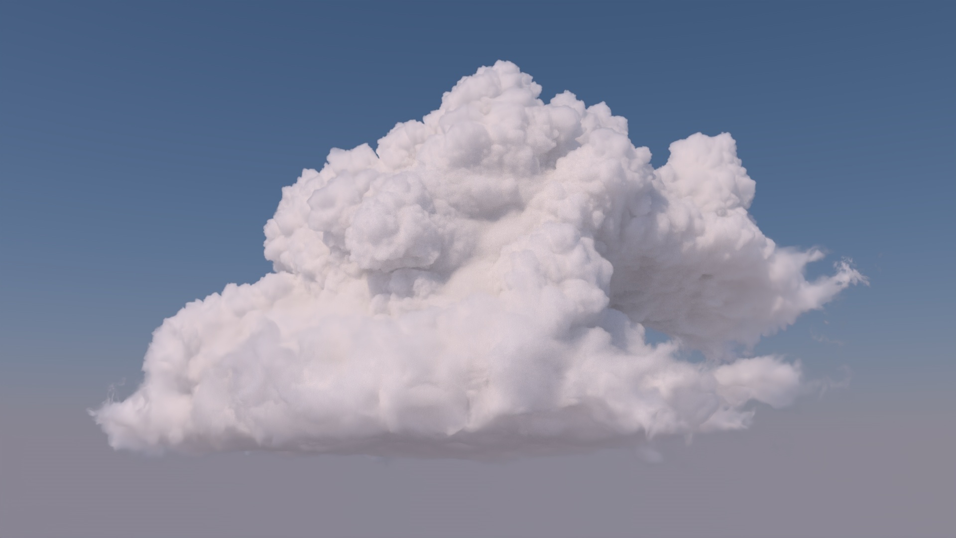
Now that everything is set, you can kick off a render and see the final imagecloud, which should look something like this: