...
Volume Settings
Max Path Length
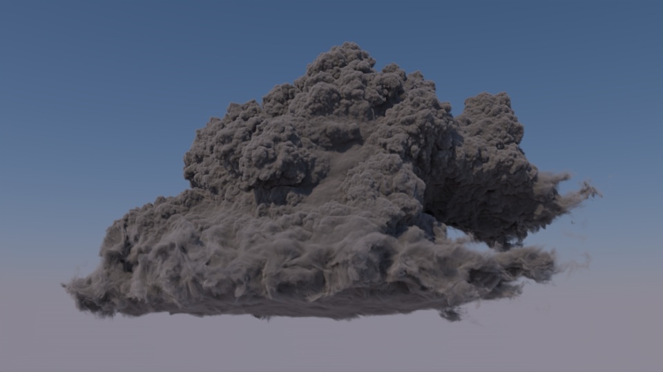
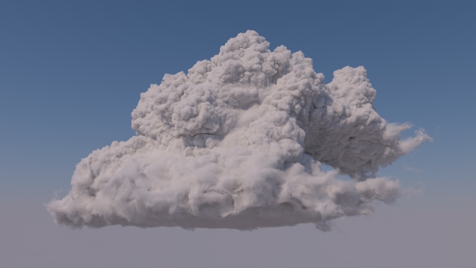
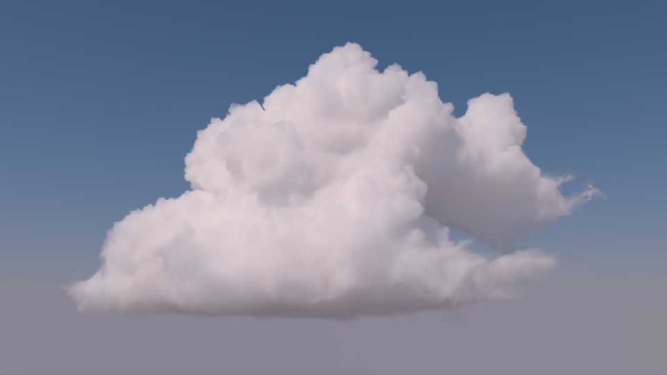
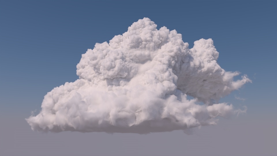
Adjusting the maximum The max path length of the integrator is critical to getting a cloudlike appearance from a render. When rendering clouds, a is an extremely important control when rendering clouds. A relatively high maximum path length is required to achieve a cloudlike appearance. The comparison images below show the Moana cloud are rendered with max path lengths of 10, 4, 16, and 64, respectively.


Notice that in addition to the cloud becoming brighter as the path length increases, the cloud rendered at path length 64 also has a silver lining that contributes to its cloudlike appearance.
However, increasing the path length can also obscure details of the cloud which are in the shadows, shown in this image rendered with path length 256. Notice that the dark areas of the cloud have less visible detail compared to the images above.

In my testing, I found that a path length of 64 was enough to replicate the look provided by increasing the path length further, so all subsequent testing uses a max path length of 64.
MSApprox

The change at higher path lengths is more subtle, but in order to get noticeable light bleed in shadowed areas of the cloud, a very high maximum path length is needed. The comparison below shows the cloud at path lengths of 64 (left) and 256 (right).
| Before After Image Slider | ||||||||||
|---|---|---|---|---|---|---|---|---|---|---|
|
| Tip |
|---|
Increasing the max path length also increases render times, so you should keep it as low as possible. Multi-Scattering Approximation (outlined below) can help mimic high path lengths at much lower cost. |
Multi-Scattering Approx
The Multi-Scattering Approximation (MS Approx) settings are a group of settings that The MSApprox settings attempt to mimic the effect of multi-scattering within a volume. When set correctly, MS Approx can produce a similar look to very high path lengths, but without increasing render times. There are three controls related to MSApprox (assuming it is enabled on the integrator). The first is the msApprox parameter on the light, which simply scales the effect of MSApprox from the light. I didn't find this parameter particularly useful, so I don't discuss it here. The other two parameters are the bleed (msApproxBleed) and contribution (msApproxContribution), which are controlled on a per-light basis. Although bleed and contribution are both colors, I will be treating them as scalars which are just the value of all three components (i.e. 0.5 is (0.5, 0.5, 0.5)). Both parameters provide an overall brightening effect on a volume, but are different in subtle ways. Balancing the bleed and contribution correctly can help approximate the look of a higher path length, but with a negligible performance impact. In my experience, enabling MSApprox with the settings that mimic higher path lengths requires reducing the brightness of the light source to prevent overexposure of the brighter areas of a volume, and all renders in this section have the light exposure changed from 0 to -1.
Bleed
The bleed parameter is important for controlling the overall brightness of a volume. Its impact is most noticeable in the darker shadows, where it can increase the brightness dramatically, but it also affects bright areas. In the below images, I fixed contribution to 0.9 (a value I found to work well with this dataset and light source), and used bleeds of 0.05, 0.15, and 0.25. In this case, a bleed of 0.15 very closely matches the look of the image above that was rendered with path length 256.


Contribution
The contribution in MSApprox The contribution parameter is particularly useful when rendering clouds because it mainly brightens central areas of a volume, leaving the edges at their original brightness. As such, I found that fairly high values of contribution could be used while still preserving the silver lining. The below images were rendered with bleed set to 0.15, and have contribution set to 0.8, 0.9, and 0.95, respectively.


Tips for MSApprox
The controls for MSApprox can be somewhat annoying, so here are some tips that might be useful for adjusting settings (specifically for clouds):
- You may have to decrease the brightness of the light when enabling MSApprox.
- Contribution is the main cause of excessive brightness, so if you are using a low contribution, this is probably unnecessary.
- Increasing contribution makes central areas brighter but not edges.
- If you're using a high contribution, adjust in very small increments (like 0.05 or less!).
- Increasing bleed mainly brightens shadowed areas.
- I found that higher bleed images needed longer to converge before the image became an accurate representation of the final render.
- It seems that bleed can be adjusted in fairly large increments without much of a problem.
- The process I used to match a look with MSApprox was:
- Start with high contribution (~0.95) and low bleed (0.1).
- Reduce contribution until the balance of edge and center brightness was right.
- Increase bleed until the overall cloud brightness looked correct.
- Both MSApprox controls are highly dependent on each other, so they need to be tuned in tandem.
Density
Density is another control that can significantly impact the look of a volume. It can be controlled by setting the densityMult on a volume. Lower multipliers will make the volume look airier (less dense) while higher values will create a more solid appearance. The following images were rendered with density multipliers of 0.0004, 0.004, and 0.01.


Anisotropy
The anisotropy of the volumes is controlled by the g0, g1, and blend of the shader, and control whether (and how) light is scattered directionally. The visual impact is difficult describe, but , which were rendered with a blend of 1 and g1 values of 0, 0.4, 0.6, and 0.8, respectively. Increasing anisotropy mainly impacts the edges and shadowed areas of the volume.


It is also possible to add a second lobe, which can be used to add some backscattering, which can help bring back detail that might be lost when anisotropy is used. The below image is rendered with a blend of 0.8, g0 set to -0.6, and g1 set to 0.8. Notice how adding the backscattering lobe helps return some of the detail that is lost when the anisotropy is increased.

Scene Setup
This section covers how to set up the scene above in some DCCs.
RfM
MS Approx controls, Multi-Scattering Approximation, MS Approx Bleed, and MS Approx Contribution. The effect of each setting is outlined in the sections below. Although Bleed and Contribution are both colors, the sections below refer to them by a single value which is used for red, green, and blue.
Multi-Scattering Approx.
The Multi-Scattering Approx. enables or disables Multi-Scattering Approximation on a light. You should set this to 1 and adjust the Bleed and Contribution settings to achieve the desired effect. Setting this to values other than 0 (disabled) or 1 (enabled) might not produce the desired effect.
| Before After Image Slider | ||||||||||
|---|---|---|---|---|---|---|---|---|---|---|
|
The cloud scene rendered with Multi-Scattering Approx. set to 0 (left) and 1 (right) with default Bleed and Contribution.
MS Approx Bleed
The MS Approx Bleed parameter controls how much light bleeds through a volume. Higher Bleed values allow more light to pass through the volume and light areas that would otherwise be shadowed. As such, the effect of MS Approx Bleed is most visible in shadowed areas of a volume, but it also creates a slight overall brightening effect. You can use the bleed parameter to compensate for the overall loss of brightness caused by lower Max Path Lengths.
| Before After Image Slider | ||||||||||
|---|---|---|---|---|---|---|---|---|---|---|
|
The cloud scene rendered with Bleed set to 0.1 (left) and 0.9 (right) with default Contribution.
| Warning |
|---|
Setting Multi-Scattering Approx to values other than 0 or 1 may not produce visually correct images |
MS Approx Contribution
The MS Approx Contribution parameter controls how much the light bleed from the Bleed parameter contributes to the brightness of the volume. Increasing Contribution tends to increase the overall brightness of the cloud, but it brightens fringes slightly less. You can use the Contribution to help bring out detail along the edges of a volume.
| Before After Image Slider | ||||||||||
|---|---|---|---|---|---|---|---|---|---|---|
|
The cloud scene rendered with Contribution set to 0.25 (left) and 0.75 (right) with default Bleed.
MS Approx Suggestions
- It can be tricky to find good values of Bleed and Contribution since they are very dependent on each other. One process you can try is to start by setting Multi-Scattering Approx to 1, then alternate increasing Contribution and decreasing Bleed in small steps until you get the correct balance of brightness in the shadowed areas.
- Contribution tends to produce a stronger brightening effect, so it should be adjusted in smaller increments than Bleed.
- At high values, the Contribution parameter becomes very sensitive, so you should adjust it in small increments (0.05 or less) as it gets close to 1.
Density
The density of a cloud has a significant impact on it's appearance. The main control for density is the Density Scale setting on the volume, which scales the density from the input OpenVDB file. Low Density Scale values create an airier, less detailed appearance with more light bleed, while high Density Scale values produce a thicker, more detailed, or even solid appearance.
The cloud scene rendered at Density Scales of 0.2 (left), 1.0 (middle), and 5.0 (right).
Anisotropy
Adjusting the anisotropy settings in PxrVolume is also critical for getting a realistic cloud render. There are three anisotropy settings to pay attention to, Primary Anisotropy, Secondary Anisotropy, and Lobe Blend Factor. The Primary and Secondary Anisotropy settings control two anisotropic lobes that can be either forward scattering (set to +1) or backward scattering (set to -1). The Lobe Blend controls the relative contribution of the two lobes, where 0 uses only the Primary lobe and 1 uses only the Secondary lobe. Setting the Primary lobe to be forward scattering flattens out detail in some areas of the cloud, but it also adds a darkening effect to parts of the cloud facing the light source.
| Before After Image Slider | ||||||||||
|---|---|---|---|---|---|---|---|---|---|---|
|
The cloud scene rendered without anisotropy (left) and with a forward scattering Primary lobe (right) with Primary Anisotropy set to 0.8 and Blend set to 0.
Adding a backward scattering Secondary lobe recovers most of the detail lost in the forward scattering render but still retains some of the detail in the areas facing the light source.
| Before After Image Slider | ||||||||||
|---|---|---|---|---|---|---|---|---|---|---|
|
The cloud scene rendered without anisotropy (left) and with a forward scattering Primary lobe and backward scattering Secondary lobe (right) with Primary Anisotropy set to 0.8, Secondary Anisotropy set to -0.2, and Blend set to 0.2.
| Note |
|---|
Enabling anisotropy will introduce additional noise to your render. Higher values of anisotropy will introduce more noise. |
Scene Setup
This section covers how the scene used above was set up in RfM.
Volume Setup
First, create an OpenVDBVisualize object from the RenderMan shelf tab.
...
In the shader settings, you can also adjust the anisotropy settings under the Anisotropy area. By default, anisotropy is off.

Light Setup
For the light setup, we will use a PxrEnvDayLight. So, the first step in the lighting setup is creating a PxrEnvDayLight from the Renderman tab of the shelf.
...
The other defaults provide a good starting point so you can leave them unchanged for now. This is also where you will adjust your MSApprox settings (under Multi-Scatter Approx). It can be quite hard to predict how MSApprox will affect the render, so you should wait to adjust these settings until after the render is set up completely.
Render Settings
The last thing we need to tweak before we see our cloud rendered is the Render Settings. So, open the Render Settings and select the RenderMan tab. The first thing you should change is under the "Aggregate Volumes" tab. For "Volume Aggregate Name", enter "globalVolumeAggregate" (this is the volume aggregate we added our cloud to before).
...
Once you set the volume aggregate name, you should see the cloud if you start a render (either in the viewport or externally in "it"), but it still won't look quite right. To give the cloud the correct appearance, we need to adjust the number of bounces. First, under "Default Ray Depth", adjust both the "Max Specular Depth" and "Max Diffuse Depth" to much higher values (e.g. no less than 32), and under "PxrPathTracer Parameters", set "Max Indirect Bounces" to that same number.

Multi-Scatter Approx
...
Now that everything is set up, you can start an IPR render from the RenderMan tab to view the cloud so we can adjust the Multi-Scatter Approx settings and see the results as we change them.
...
To begin with, go to the settings on our PxrEnvDayLight and enable MSApprox by setting "Multi-Scatter Approx" to 1. Now, you can adjust the bleed and contribution as described above. If you find that the cloud is too bright, reducing the value of the MS Approx setting from 1 is an easy way to change the brightness without having to tweak the bleed and contribution too much.

Render
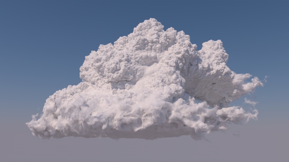
Now that everything is set, you can kick off a render and see the final image, which should look something like this:
...